2.3 What Julia Aims to Accomplish?

NOTE: In this section we will explain the details of what makes Julia shine as a programming language. If it becomes too technical for you, you can skip and go straight to Section 4 to learn about tabular data with DataFrames.jl.

The Julia programming language (Bezanson et al., 2017) is a relatively new language, first released in 2012, and aims to be both easy and fast. It “runs like C⁸ but reads like Python” (Perkel, 2019). It was made for scientific computing, capable of handling large amounts of data and computation while still being fairly easy to manipulate, create, and prototype code.

The creators of Julia explained why they created Julia in a 2012 blogpost. They said:

We are greedy: we want more. We want a language that’s open source, with a liberal license. We want the speed of C with the dynamism of Ruby. We want a language that’s homoiconic, with true macros like Lisp, but with obvious, familiar mathematical notation like Matlab. We want something as usable for general programming as Python, as easy for statistics as R, as natural for string processing as Perl, as powerful for linear algebra as Matlab, as good at gluing programs together as the shell. Something that is dirt simple to learn, yet keeps the most serious hackers happy. We want it interactive and we want it compiled.

Most users are attracted to Julia because of the superior speed. After all, Julia is a member of a prestigious and exclusive club. The petaflop club is comprised of languages who can exceed speeds of one petaflop⁹ per second at peak performance. Currently only C, C++, Fortran, and Julia belong to the petaflop club.

But, speed is not all that Julia can deliver. The ease of use, Unicode support, and a language that makes code sharing effortless are some of Julia’s features. We’ll address all those features in this section, but we want to focus on the Julia code sharing feature for now.

The Julia ecosystem of packages is something unique. It enables not only code sharing but also allows sharing of user-created types. For example, Python’s pandas uses its own Datetime type to handle dates. The same with R tidyverse’s lubridate package, which also defines its own datetime type to handle dates. Julia doesn’t need any of this, it has all the date stuff already baked into its standard library. This means that other packages don’t have to worry about dates. They just have to extend Julia’s DateTime type to new functionalities by defining new functions and do not need to define new types. Julia’s Dates module can do amazing stuff, but we are getting ahead of ourselves now. Let’s talk about some other features of Julia.

2.3.1 Julia Versus Other Programming Languages

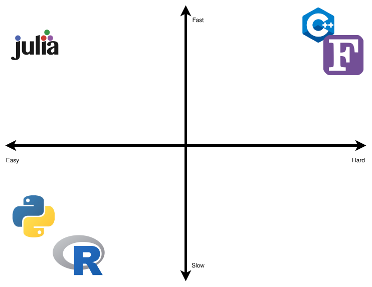
In Figure 2, a highly opinionated representation is shown that divides the main open source and scientific computing languages in a 2x2 diagram with two axes: Slow-Fast and Easy-Hard. We’ve omitted closed source languages because there are many benefits to allowing other people to run your code for free as well as being able to inspect the source code in case of issues.

We’ve put C++ and FORTRAN in the hard and fast quadrant. Being static languages that need compilation, type checking, and other professional care and attention, they are really hard to learn and slow to prototype. The advantage is that they are really fast languages.

R and Python go into the easy and slow quadrant. They are dynamic languages that are not compiled and they execute in runtime. Because of this, they are really easy to learn and fast to prototype. Of course, this comes with a disadvantage: they are really slow languages.

Julia is the only language in the easy and fast quadrant. We don’t know any other serious language that would want to be hard and slow, so this quadrant is left empty.

Julia is fast! Very fast! It was designed for speed from the beginning. In the rest of this section, we go into details about why this is. If you don’t have (much) programming experience yet, feel free to skip to the next section and maybe come later to this at a later moment.

Julia accomplishes it’s speed partially due to multiple dispatch. Basically, the idea is to generate very efficient LLVM¹⁰ code. LLVM code, also known as LLVM instructions, are very low-level, that is, very close to the actual operations that your computer is executing. So, in essence, Julia converts your hand written and easy to read code to LLVM machine code which is very hard for humans to read, but easy for computers to read. For example, if you define a function taking one argument and pass an integer into the function, then Julia will create a specialized MethodInstance. The next time that you pass an integer to the function, Julia will look up the MethodInstance that was created earlier and refer execution to that. Now, the great trick is that you can also do this inside a function that calls a function. For example, if some data type is passed into function outer and outer calls function inner and the data types passed to inner are known inside the specialized outer instance, then the generated function inner can be hardcoded into function outer! This means that Julia doesn’t even have to lookup MethodInstances any more, and the code can run very efficiently.

Let’s show this in practice. We can define the two functions, inner:

inner(x) = x + 3

and outer:

outer(x) = inner(2 * x)

For example, we can now calculate outer for, let’s say, 3:

outer(3)

9

If you step through this calculation of outer, you’ll see that the program needs do do quite a lot of things:

1. calculate 2 * 3
2. pass the outcome of 2 * 3 to inner
3. calculate 3 + the outcome of the previous step

But, if we ask Julia for the optimized code via @code_typed, we see what instructions the computer actually get:

@code_llvm debuginfo=:none outer(3)

define i64 @julia_outer_232(i64 signext %0) #0 {
top:
  %1 = shl i64 %0, 1
  %2 = add i64 %1, 3
  ret i64 %2
}

This is low-level LLVM code showing that the program only does the following:

1. shift the input (3) one bit to the left, which has the same effect as multiplying by 2; and
2. add 3.

and that’s it! Julia has realized that calling inner can be removed, so that’s not part of the calculation anymore! Now, imagine that this function is called a thousand or even a million times. These optimizations will reduce the running time significantly.

The trade-off, here, is that there are cases where earlier assumptions about the hardcoded MethodInstances are invalidated. Then, the MethodInstance has to be recreated which takes time. Also, the trade-off is that it takes time to infer what can be hardcoded and what not. This explains why it can often take very long before Julia does the first thing: in the background, it is optimizing your code.

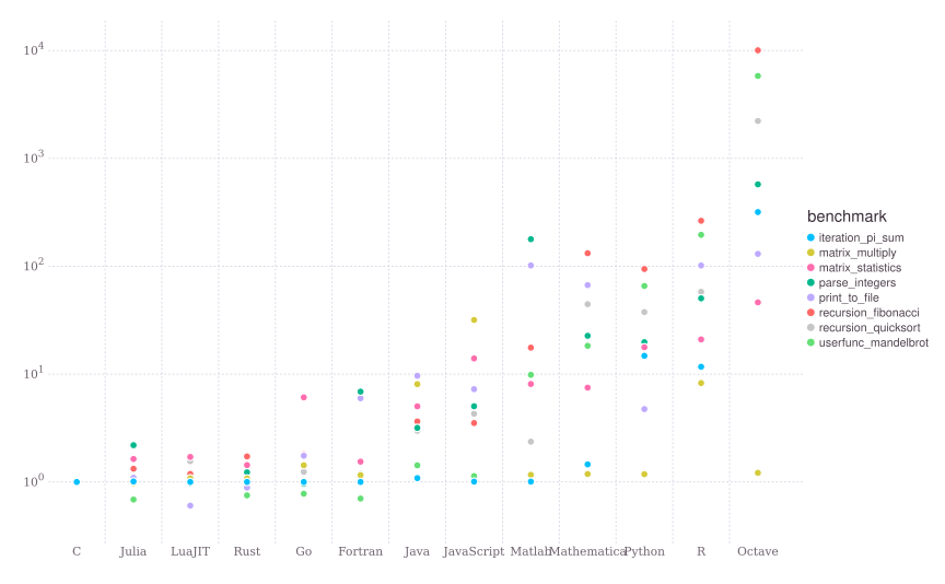
So, Julia creates optimized LLVM machine code¹¹. You can find benchmarks for Julia and several other languages here. Figure 3 was taken from Julia’s website benchmarks section¹². As you can see Julia is indeed fast.

We really believe in Julia. Otherwise, we wouldn’t be writing this book. We think that Julia is the future of scientific computing and scientific data analysis. It enables the user to develop rapid and powerful code with a simple syntax. Usually, researchers develop code by prototyping using a very easy, but slow, language. Once the code is assured to run correctly and fulfill its goal, then begins the process of converting the code to a fast, but hard, language. This is known as the “Two-Language Problem” and we discuss next.

2.3.2 The Two-Language Problem

The “Two-Language Problem” is a very typical situation in scientific computing where a researcher devises an algorithm or a solution to tackle a desired problem or analysis at hand. Then, the solution is prototyped in an easy to code language (like Python or R). If the prototype works, the researcher would code in a fast language that would not be easy to prototype (C++ or FORTRAN). Thus, we have two languages involved in the process of developing a new solution. One which is easy to prototype but is not suited for implementation (mostly due to being slow). And another which is not so easy to code, and consequently not easy to prototype, but suited for implementation because it is fast. Julia avoids such situations by being the same language that you prototype (ease of use) and implement the solution (speed).

Also, Julia lets you use Unicode characters as variables or parameters. This means no more using sigma or sigma_i, and instead just use \(σ\) or \(σᵢ\) as you would in mathematical notation. When you see code for an algorithm or for a mathematical equation, you see almost the same notation and idioms. We call this feature “One-To-One Code and Math Relation” which is a powerful feature.

We think that the “Two-Language problem” and the “One-To-One Code and Math Relation” are best described by one of the creators of Julia, Alan Edelman, in a TEDx Talk (TEDx Talks, 2020).

2.3.3 Multiple Dispatch

Multiple dispatch is a powerful feature that allows us to extend existing functions or to define custom and complex behavior for new types. Suppose that you want to define two new structs to denote two different animals:

abstract type Animal end
struct Fox <: Animal
    weight::Float64
end
struct Chicken <: Animal
    weight::Float64
end

Basically, this says “define a fox which is an animal” and “define a chicken which is an animal”. Next, we might have one fox called Fiona and a chicken called Big Bird.

fiona = Fox(4.2)
big_bird = Chicken(2.9)

Next, we want to know how much they weight together, for which we can write a function:

combined_weight(A1::Animal, A2::Animal) = A1.weight + A2.weight

combined_weight (generic function with 1 method)

And we want to know whether they go well together. One way to implement that is to use conditionals:

function naive_trouble(A::Animal, B::Animal)
    if A isa Fox && B isa Chicken
        return true
    elseif A isa Chicken && B isa Fox
        return true
    elseif A isa Chicken && B isa Chicken
        return false
    end
end

naive_trouble (generic function with 1 method)

Now, let’s see whether leaving Fiona and Big Bird together would give trouble:

naive_trouble(fiona, big_bird)

true

Okay, so this sounds right. Writing the naive_trouble function seems to be easy enough. However, using multiple dispatch to create a new function trouble can have their benefits. Let’s create our new function as follows:

trouble(F::Fox, C::Chicken) = true
trouble(C::Chicken, F::Fox) = true
trouble(C1::Chicken, C2::Chicken) = false

trouble (generic function with 3 methods)

After defining these methods, trouble gives the same result as naive_trouble. For example:

trouble(fiona, big_bird)

true

And leaving Big Bird alone with another chicken called Dora is also fine

dora = Chicken(2.2)
trouble(dora, big_bird)

false

So, in this case, the benefit of multiple dispatch is that you can just declare types and Julia will find the correct method for your types. Even more so, for many cases when multiple dispatch is used inside code, the Julia compiler will actually optimize the function calls away. For example, we could write:

function trouble(A::Fox, B::Chicken, C::Chicken)
    return trouble(A, B) || trouble(B, C) || trouble(C, A)
end

Depending on the context, Julia can optimize this to:

function trouble(A::Fox, B::Chicken, C::Chicken)
    return true || false || true
end

because the compiler knows that A is a Fox, B is a chicken and so this can be replaced by the contents of the method trouble(F::Fox, C::Chicken). The same holds for trouble(C1::Chicken, C2::Chicken). Next, the compiler can optimize this to:

function trouble(A::Fox, B::Chicken, C::Chicken)
    return true
end

Another benefit of multiple dispatch is that when someone else now comes by and wants to compare the existing animals to their animal, a Zebra, then that’s possible. In their package, they can define a Zebra:

struct Zebra <: Animal
    weight::Float64
end

and also how the interactions with the existing animals would go:

trouble(F::Fox, Z::Zebra) = false
trouble(Z::Zebra, F::Fox) = false
trouble(C::Chicken, Z::Zebra) = false
trouble(Z::Zebra, F::Fox) = false

trouble (generic function with 6 methods)

Now, we can see whether Marty (our zebra) is safe with Big Bird:

marty = Zebra(412)
trouble(big_bird, marty)

false

Even better, we can also calculate the combined weight of zebra’s and other animals without defining any extra function at our side:

combined_weight(big_bird, marty)

414.9

So, in summary, the code that was written with only Fox and Chicken in mind works even for types that it has never seen before! In practice, this means that Julia makes it often easy to re-use code from other projects.

If you are excited as much as we are by multiple dispatch, here are two more in-depth examples. The first is a fast and elegant implementation of a one-hot vector by Storopoli (2021). The second is an interview with Christopher Rackauckas at Tanmay Bakshi YouTube’s Channel (see from time 35:07 onwards) (tanmay bakshi, 2021). Chris mentions that, while using DifferentialEquations.jl, a package that he developed and currently maintains, a user filed an issue that his GPU-based quaternion ODE solver didn’t work. Chris was quite surprised by this request since he would never have expected that someone would combine GPU computations with quaternions and solving ODEs. He was even more surprised to discover that the user made a small mistake and that it all worked. Most of the merit is due to multiple dispatch and high user code/type sharing.

To conclude, we think that multiple dispatch is best explained by one of the creators of Julia: Stefan Karpinski at JuliaCon 2019.